CUDA Matmul (Part 1): Naive GPU vs CPU implementation and benchmarking

This post explores matrix multiplication (matmul) on GPU, starting with a simple sequential CPU implementation as our baseline. We then demonstrate how GPU parallelization can be achieved by utilizing individual threads for computation. Finally, we compare the performance of both implementations through benchmarks measuring GFLOPS, execution time, and speedup.

The following GPU implementation will be used in future posts of this series, and will act as a benchmark against more optimized GPU implementations.

Sequential CPU Implementation

Let’s start with our CPU baseline - a straightforward single-threaded implementation:

void cpu_matmul(
    const float *mat_A, const float *mat_B, float *mat_C,
    int M, int N, int K
    )
{
    for (int i = 0; i < M; i++) {
        for (int j = 0; j < N; j++) {
            float sum = 0.0f;
            for (int k = 0; k < K; k++) {
                sum += mat_A[idx(i, k, K)] * mat_B[idx(k, j, N)];
            }
            mat_C[idx(i, j, N)] = sum;
        }
    }
}

This implementation computes the result sequentially using three nested loops, processing one element of the output matrix at a time.

For each element $C[i,j]$ in the output matrix, we compute the dot product between row $i$ of matrix $A$ and column $j$ of matrix $B$. As we will see, this sequential approach is significantly slower than parallel GPU implementations that can compute many elements simultaneously.

As aforementioned, this post seeks to focus on first introducing a naive GPU version. This version is far from optimal, but serves as a starting point for further optimizations.

Naive GPU Matrix Multiplication Explained by Example

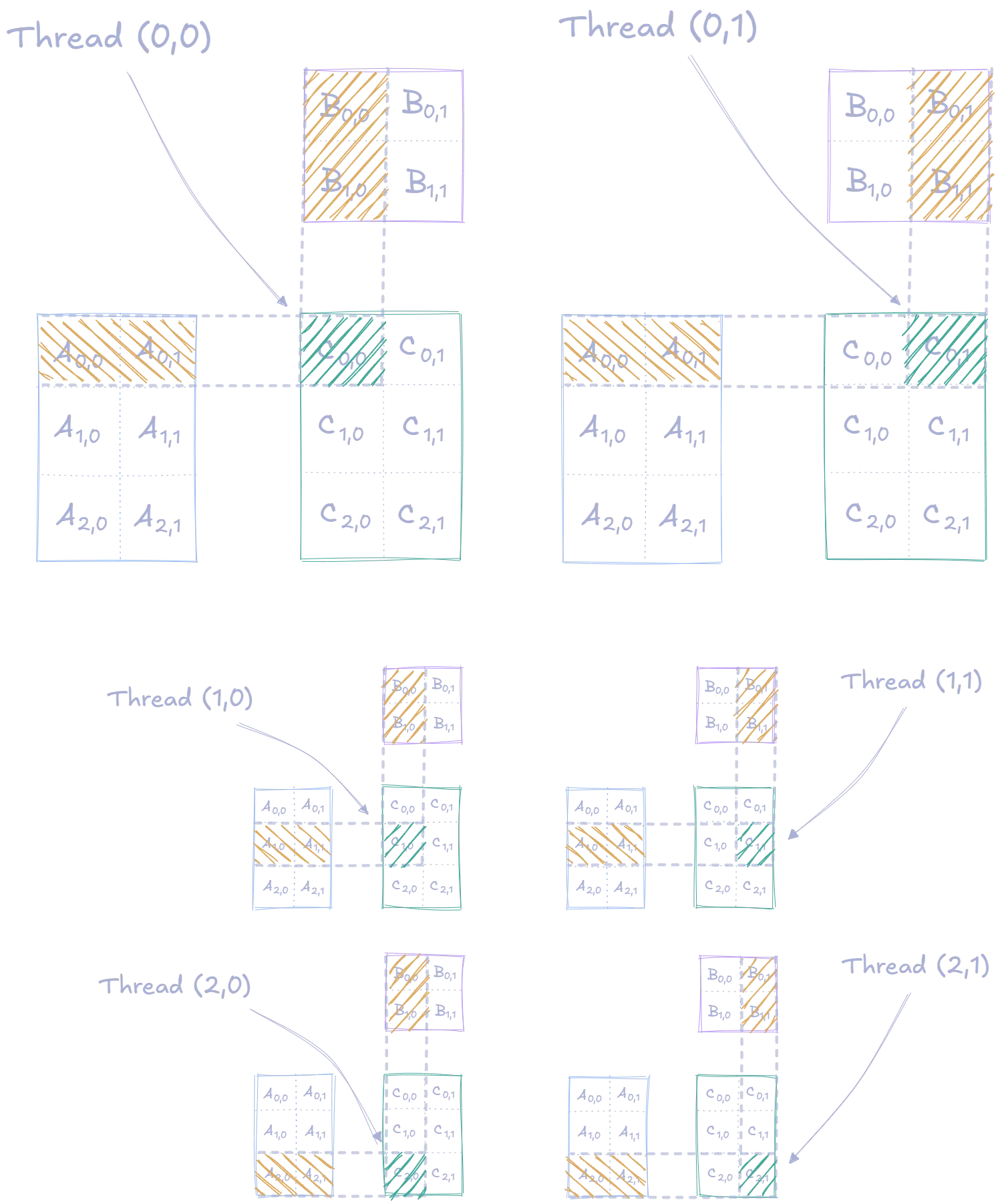
Matrix multiplication is particularly well-suited for GPU acceleration due to the independent nature of computing each output element. For our initial GPU implementation, we will take the most straightforward approach: assigning each output element to a dedicated CUDA thread.

Thus, each thread in this implementation needs to:

1. Determine which output element it’s responsible for using its thread and block indices
2. Compute that element by performing the necessary dot-product calculation between the corresponding row of $A$ and column of $B$

For our example, we will multiply two matrices $A$ and $B$ of size $3 \times 2$ and $2 \times 2$, resulting in a matrix $C$ of size $3 \times 2$. All three matrices are stored in global memory. This is one of the main bottlenecks of this approach, as global memory is slower bandwidth and higher latency than other memory hierarchy levels. However, this is an optimization for future posts of this series. Moving on, the matrices are depicted below:

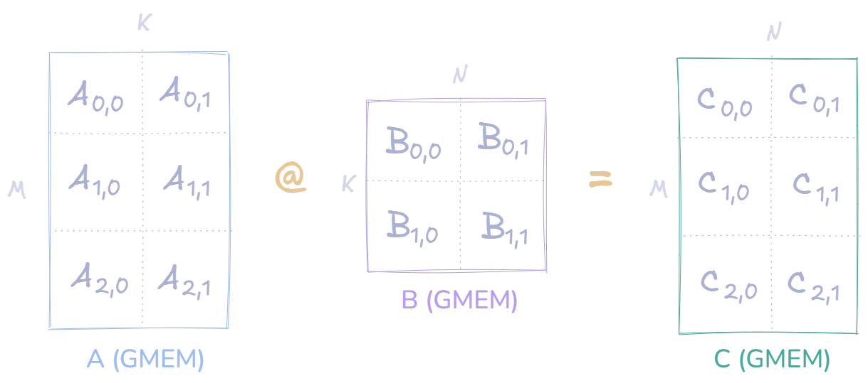
With this approach, the entire computation of the output matrix $C$ requires $6$ threads, with each thread handling one element. The assignment of threads to elements is depicted in the following image:

Before looking at the implementation, it’s important to understand how threads are organized. CUDA uses a hierarchical threading model where threads are grouped into blocks, which are then organized into a grid.

In our implementation, we use 16×16 thread blocks, meaning each block contains 256 threads arranged in a 2D pattern. For our example matrix $C$ of size $3 \times 2$:

• We only need 6 threads for the computation
• However, we launch a full block of $16 \times 16$ threads
• We use boundary checks to ensure we aren’t accessing memory out of bounds, so only the needed are ‘active’
• The remaining threads are ‘idle’

The image below shows the active threads in the $16 \times 16$ block that our threads grouped into:

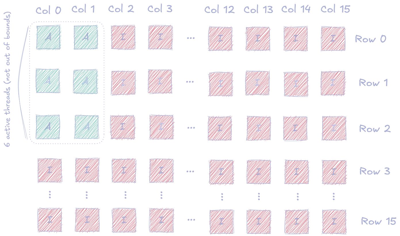
Since our matrix $C$ is only of size $3 \times 2$, we only need 1 block of $16 \times 16$ threads. Conversely, for a matrix of size $32 \times 32$:

• We would need $32 \times 32 = 1024$ threads in total
• Each block has $256$ threads
• So the number of blocks needed = $1024 \div 256 = 4$ (fully occupied)
• These would then be arranged into a $2 \times 2$ grid of blocks to match the shape of our output matrix

Let’s visualize this to gain some intuition:

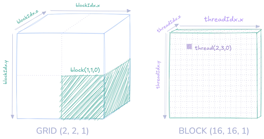
This corresponds to the following code:

int N = 32, M = 32;

dim3 block_size(16, 16);
dim3 grid_size(
    (N + block_size.x - 1) / block_size.x, // 2 blocks in x direction
    (M + block_size.y - 1) / block_size.y  // 2 blocks in y direction
);

When passed to a kernel launch configuration, this creates a $2 \times 2 \times 1$ grid of blocks ($z$ defaults to $1$), with each block grouping $16 \times 16 \times 1$ threads (again, $z$ defaults to $1$).

As aforementioned, this is enough to parallelize the computation of the entire $32 \times 32$ matrix output matrix, as depicted below:

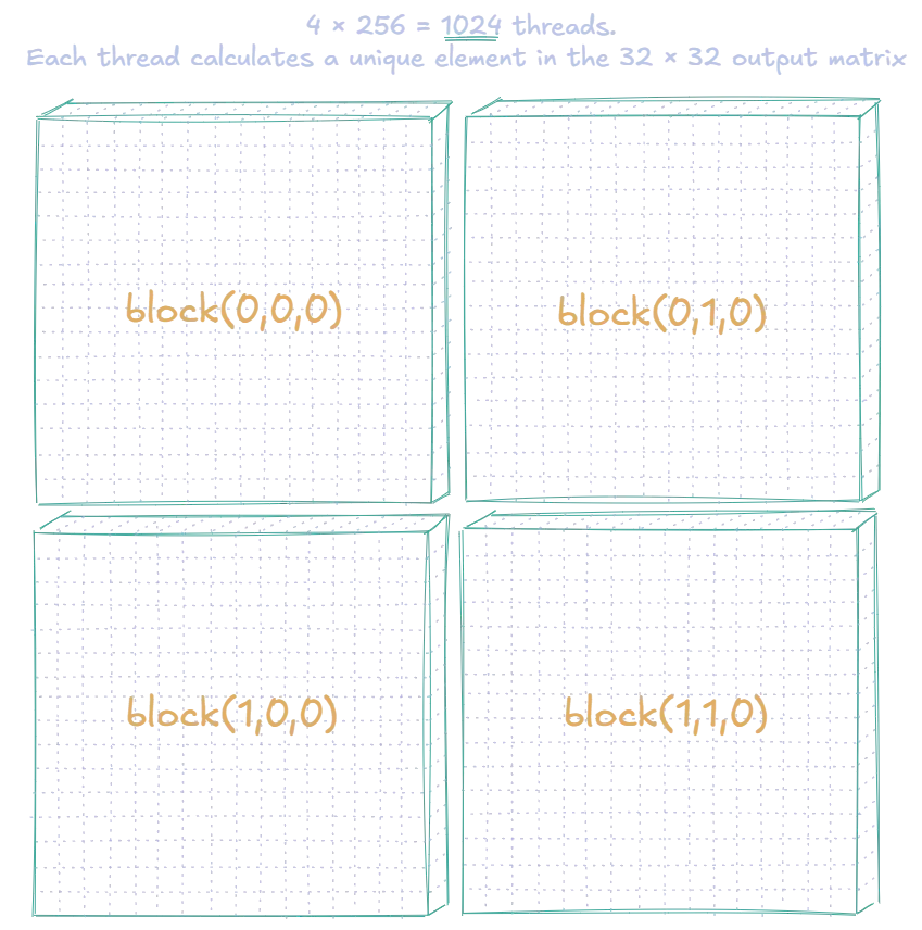
One could imagine a significant speedup by having 1024 threads computing unique elements of the output matrix in parallel, compared to the sequential CPU implementation. We will confirm this later in the benchmarking section.

First, let’s see how this could be implemented in CUDA.

Naive GPU Matrix Multiplication Implementation

Let’s see look at how this approach can be implemented in CUDA. Here’s the kernel code:

__global__ void naive_matmul_kernel(
  const float* mat_A, const float* mat_B, float* mat_C,
  int M, int N, int K
  )
{
  int row = blockIdx.y * blockDim.y + threadIdx.y;
  int col = blockIdx.x * blockDim.x + threadIdx.x;

  if (row < M && col < N) {
    float cell_sum = 0.0f;

    for(int k = 0; k < K; k++) {
      cell_sum += mat_A[idx(row, k, K)] * mat_B[idx(k, col, N)];
    }

    mat_C[idx(row, col, N)] = cell_sum;
  }
}

Let’s examine the key components:

Each thread is responsible for calculating its own position in the output matrix $C$. This position is defined by a row and column index, which can be calculated using the built-in CUDA variables:

• threadIdx.x, threadIdx.y and threadIdx.z to get a threads position within its block
• blockIdx.x, blockIdx.y and blockIdx.z to get a blocks position within its grid

In case you skipped it, you might find this image useful for getting a grasp of the above.

The calculations are as follows:

row = blockIdx.y * blockDim.y + threadIdx.y
col = blockIdx.x * blockDim.x + threadIdx.x

For example $thread(2,1)$ in $block(0,0)$ would compute its row by $0 \times 16 + 2 = 2$ and its column by $0 \times 16 + 1 = 1$.

if (row < M && col < N) { ... }

This if-statement is a boundary check to ensure we only compute elements within the bounds of matrix dimensions, since we might launch more threads than we actually need. A scenario with a block containing inactive threads was also depicted earlier in this image.

for(int k = 0; k < K; k++) {
  cell_sum += mat_A[idx(row, k, K)] * mat_B[idx(k, col, N)];
}

Each thread simply computes the dot product of its computed $row$ of $A$ and its computed $col$ of $B$. Note that all the accesses in matrices $A$ and $B$ are global accesses, which is a performance bottleneck. This will be addressed in the next post.

Furthermore, we have the function that sets up the grid and block sizes as presented earlier, and uses them in the kernel configuration:

void naive_matmul(
  const float* mat_A, const float* mat_B, float* mat_C,
  int M, int N, int K
  )
{
  dim3 block_size(16, 16);
  dim3 grid_size(
    (N + block_size.x - 1) / block_size.x,
    (M + block_size.y - 1) / block_size.y
  ); // use ceiling division to ensure enough blocks for matrix dimensions


  naive_matmul_kernel<<<grid_size, block_size>>>(mat_A, mat_B, mat_C, M, N, K);

}

Now that we have implemented both sequential CPU and naive GPU versions, we can compare their performance. As our GPU implementation parallelizes the computation across many threads, we expect to see significant speedup over the sequential CPU version, especially for larger matrices.

Benchmarking: Sequential CPU vs Naive GPU

The table below includes the results from benchmarking the implementation for different matrix sizes. These benchmarks were run on an NVIDIA A10, and an AMD EPYC-Milan CPU.

The difference in performance between the different matrix sizes demonstrates how well GPU parallelism can scale with problem size. Notably, $1024 \times 1024$ receives the largest speedup of 2600.7× and 860.85 GFLOPS, as the GPU can better utilize the available threads.

Even for smaller matrices a decent speedup is achieved, however the GPU’s parallelism is left underutilized.

Conclusion

While these speedups are significant, our naive implementation still has considerable room for improvement. Each thread repeatedly accesses global memory, and our memory access patterns aren’t optimized for the GPU memory hierarchy. Therefore, the next post posts will consider:

• Tiled matrix multiplication, which allows for a number of reuse patterns
• Shared memory utilization to reduce the number of global memory accesses, allowing for lower latency and higher bandwidth
• NVIDIA NSight Compute to profile the more optimized implementations against the naive GPU implementation, to gain insights on memory access patterns and cache utilization (L1 and L2)