CUDA Matmul (Part 2): Understanding Tiled Matrix Multiplication - Benchmarking, and Profiling

In the previous post we implemented a naive GPU matrix multiplication implementation, where each thread was responsible for calculating a single element in the output matrix. A benchmark was then conducted against a sequential CPU implementation, and we saw a $2600.7 \times$ speedup for a $1024 \times 1024$ matrix, reaching $860.85$ GFLOPS:

In the naive GPU implementation, each thread repeatedly accessed global memory for every multiplication operation, leading to high memory latency and inefficient bandwidth utilization.

The goal of this post is to implement, benchmark and profile an optimization that can be done to further improve our previous naive GPU implementation.

Tiled Matrix Multiplication Explained by Example

In our previous implementation, each thread independently accessed global memory to compute its elements of the output matrix. This resulted in redundant memory accesses and inefficient use of the GPU’s memory bandwidth. Tiled matrix multiplication addresses this by having threads cooperate to load data into shared memory. Shared memory is located on-chip, and as such has a much lower latency and higher bandwidth compared to global memory.

I was not able to find the shared memory bandwidth for the Ampere architecture explicitly stated anywhere. However, a benchmark from this paper for the Volta architecture shows:

• Global memory bandwidth: $750$ GiB/s
• Shared memory bandwidth: $120,080$ GiB/s

Let’s examine how this tiled matrix multiplication works step by step. The diagram below shows matrices A and B in global memory (GMEM) on the left. For efficiency, we don’t want to constantly access this slower global memory, so we load small tiles of each matrix into much faster shared memory (SMEM)

For the sake of simplicity, $A$ and $B$ are $4 \times 4$ matrices, and we use a $2 \times 2$ tile size for our example. We will focus on the computation performed by thread Block(0,0), which is responsible for calculating the upper-left region of matrix $C$.

First, all threads in Block(0,0) participate in loading the tiles into shared memory. Each thread in the block attempts to load one element from $A$ and one from $B$ into shared memory:

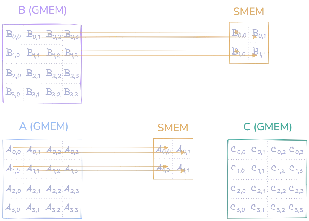
These loaded tiles are then used to compute partial results for the upper-left region of matrix $C$. We first compute $A_{0,0} \times B_{0,0}$ for the partial result of $C_{0,0}$, $A_{0,0} \times B_{0,1}$ for the partial result of $C_{0,1}$, and so on:

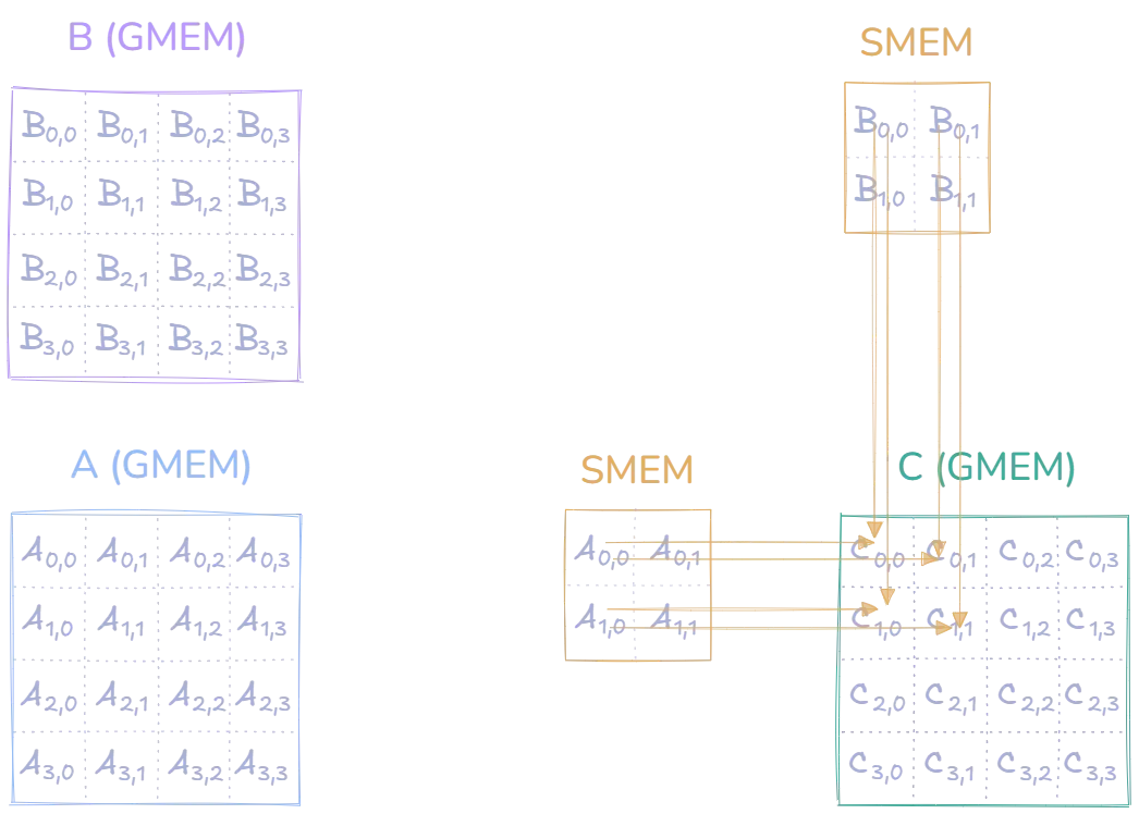
Looking at the diagram, it might seem like we have everything needed to compute the final values of $C$‘s upper-left region, but we’re actually only seeing one step. Let’s take $C_{0,0}$ as an example. To compute $C_{0,0}$, we need to compute the dot product of row 0 of $A$ and column 0 of $B$. Writing this out we get:

$$C_{0,0} = (A_{0,0} \times B_{0,0} + A_{0,1} \times B_{1,0}) + (A_{0,2} \times B_{2,0} + A_{0,3} \times B_{3,0})$$

So far, the loaded tiles only lets us compute the first part in parentheses: $(A_{0,0} \times B_{0,0} + A_{0,1} \times B_{1,0})$. Focusing on $C_{0,0}$, we can still do a second multiplication $A_{0,1} \times B_{1,0}$ and add it to the result of the first multiplication before moving on and loading a new tile into shared memory. to calculate the second part in parentheses:

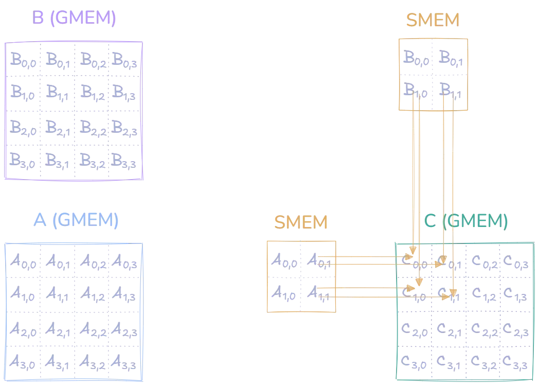
To finish the computation of $C_{0,0}$ (and the rest in the upper-left region), we need to load a set of new tiles into shared memory, and then do two more multiplications, which we add to the result of the previous multiplications:

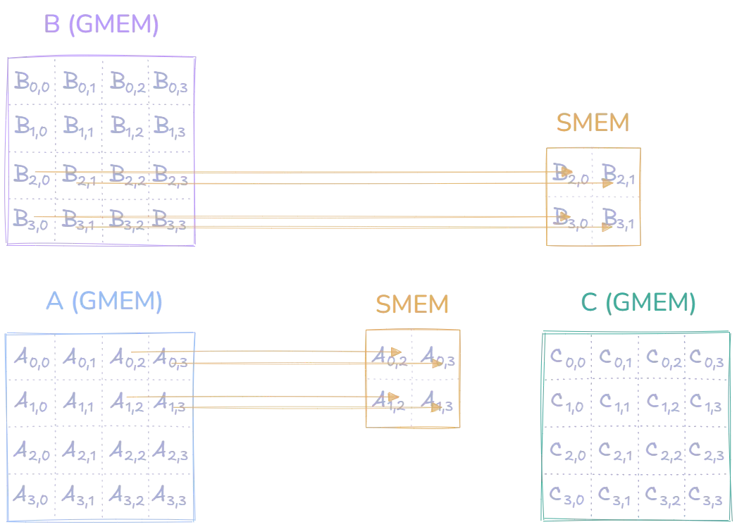
We then do the final two computations with the newly loaded tiles. This concludes the computation of $C_{0,0}, C_{0,1}$, $C_{1,0}$ and $C_{1,1}$:

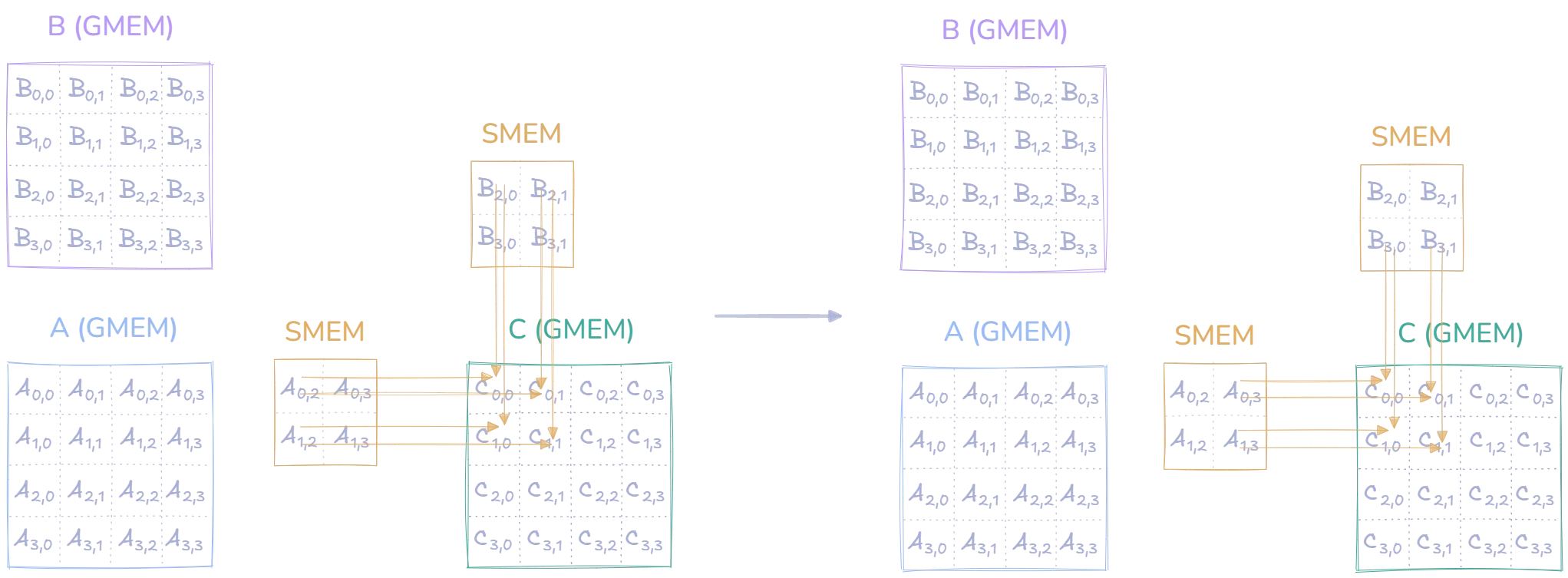
Note that this example focused on the upper-left region of $C$. These computations were performed by thread $Block(0,0)$, while other thread blocks were simultaneously computing other regions of $C$: $Block(0,1)$ handling the upper-right region, $Block(1,0)$ the lower-left region, and $Block(1,1)$ the lower-right region.

This example demonstrates the fundamental concept of tiled matrix multiplication on GPUs - loading small chunks of data into shared memory to improve memory access efficiency. Rather than having each thread repeatedly access global memory, we load tiles collaboratively and reuse data from the much faster shared memory. Each thread block handles its own region of the output matrix ($C$) in parallel, with threads within the block cooperating to load and compute their assigned tiles.

Matrix multiplication is considered a memory-bound operation, because its performance is often limited by the rate at which data can be moved between global memory and the GPU’s processing cores, rather than the speed of the computations themselves. Enabling data reuse by using shared memory can help improve the arithmetic intensity (the ratio of computations to memory accesses), allowing GPU cores to perform more work instead of waiting for data.

As such, we expect a significant improvement over the naive GPU implementation.

Tiled Matrix Multiplication Implementation

Before benchmarking, let’s first look at how one could implement tiled matrix multiplication. Below is the code for the entire kernel, we will then break it down into smaller parts:

template<int TILE_SIZE>
__global__ void tiled_matmul_kernel(
    const float* mat_A, const float* mat_B, float* mat_C,
    int M, int N, int K)
{
    __shared__ float shared_A[TILE_SIZE][TILE_SIZE];
    __shared__ float shared_B[TILE_SIZE][TILE_SIZE];

    int row = blockIdx.y * blockDim.y + threadIdx.y;
    int col = blockIdx.x * blockDim.x + threadIdx.x;

    int tx = threadIdx.x, ty = threadIdx.y;

    float sum = 0.0f;

    // loop over tiles
    for (int tile = 0; tile < (K + TILE_SIZE - 1) / TILE_SIZE; tile++) {
        // load tile from mat_A into shared memory
        if (row < M && (tile * TILE_SIZE + tx) < K) {
            int a_row = row;
            int a_col = tile * TILE_SIZE + tx;
            shared_A[ty][tx] = mat_A[idx(a_row, a_col, K)];
        } else {
            shared_A[ty][tx] = 0.0f; // pad with 0's if out of bounds
        }

        // load tile from mat_B into shared memory
        if (col < N && (tile * TILE_SIZE + ty) < K) {
            int b_row = tile * TILE_SIZE + ty;
            int b_col = col;
            shared_B[ty][tx] = mat_B[idx(b_row, b_col, N)];
        } else {
            shared_B[ty][tx] = 0.0f;
        }

        __syncthreads();  // wait for all threads to load their data
        for (int k = 0; k < TILE_SIZE; k++) {
            sum += shared_A[ty][k] * shared_B[k][tx];
        }
        __syncthreads();
    }

    // write result
    if (row < M && col < N) {
        mat_C[idx(row, col, N)] = sum;
    }
}

Let’s look at the key components that are new in this implementation.

   __shared__ float shared_A[TILE_SIZE][TILE_SIZE];
   __shared__ float shared_B[TILE_SIZE][TILE_SIZE];

These arrays are shared among all threads in a block, and they provide fast bandwidth and low latency to the tiles being processed.

int row = blockIdx.y * blockDim.y + threadIdx.y;
int col = blockIdx.x * blockDim.x + threadIdx.x;

Similar to our naive implementation, each thread calculates its position in the output matrix.

for (int tile = 0; tile < (K + TILE_SIZE - 1) / TILE_SIZE; tile++)

This loop iterates over all the tiles that are needed to compute the final result. We utilize ceiling division again, to handle matrices where $K$ is not divisible by $TILE\_SIZE$.

Relating this to the example used earlier, this outer loop corresponds to loading new values in the two $2 \times 2$ tiles used by $A$ and $B$. For instance, in our example of calculating $C_{0,0}$, we needed two iterations of this loop - one for tiles containing $(A_{0,0}, A_{0,1})$ and $(B_{0,0}, B_{1,0})$, and another for tiles containing $(A_{0,2}, A_{0,3})$ and $(B_{2,0}, B_{3,0})$.

if (row < M && (tile * TILE_SIZE + tx) < K) {
    int a_row = row;
    int a_col = tile * TILE_SIZE + tx;
    shared_A[ty][tx] = mat_A[idx(a_row, a_col, K)];
} else {
    shared_A[ty][tx] = 0.0f; // pad with 0's if out of bounds
}

Here threads do collaborative loading of tiles from $A$ into shared memory. The if statement handles the case where the matrix dimensions aren’t perfect multiples of our tile size. In our code we defined the $TILE\_SIZE$ to be $16 \times 16$, so if we have a $1030 \times 1030$ matrix, the very last tile would only need to load 6 elements in each dimension since $(1030 - 16 \cdot 64) = 6$. Therefore, we need boundary checks to ensure we aren’t accessing memory out of bounds.

The code for loading tiles from $B$ into shared memory is similar.

__synthreads();

The __syncthreads() CUDA intrinsic function is used to synchronize all threads within a block, ensuring they have all reached this point before any thread proceeds further. In the implementation it is used twice:

• The first time to ensure all threads have loaded their data into shared memory
• The second time to ensure all threads are done using the current tiles

for (int k = 0; k < TILE_SIZE; k++) {
    sum += shared_A[ty][k] * shared_B[k][tx];
}

The inner loop performs the actual matrix multiplication using the data in shared memory. Taking our earlier example of computing $C_{0,0}$: in the first iteration with loaded tiles, this loop computes $(A_{0,0} \times B_{0,0} + A_{0,1} \times B_{1,0})$, and in the second iteration with new tiles, it computes $(A_{0,2} \times B_{2,0} + A_{0,3} \times B_{3,0})$.

if (row < M && col < N) {
    mat_C[idx(row, col, N)] = sum;
}

Finally, once a thread has accumulated all partial sums (in our example, after both tiles have been processed), it writes its final result to matrix $C$ in global memory. The boundary check ensures we only write valid results when the matrix dimensions aren’t perfect multiples of our tile size.

The following host function sets up and launches the kernel:

void tiled_matmul(
    const float* mat_A, const float* mat_B, float* mat_C,
    int M, int N, int K)
{
    constexpr int TILE_SIZE = 16;

    dim3 block_size(TILE_SIZE, TILE_SIZE);
    dim3 grid_size(
        (N + block_size.x - 1) / block_size.x,
        (M + block_size.y - 1) / block_size.y
    );

    tiled_matmul_kernel<TILE_SIZE><<<grid_size, block_size>>>(
        mat_A, mat_B, mat_C, M, N, K);
}

We set TILE_SIZE to 16, creating 16×16 thread blocks. The grid size is calculated to ensure we have enough blocks to cover the entire output matrix, using ceiling division to handle matrices with dimensions that aren’t multiples of the tile size.

Benchmarking against the Naive GPU Implementation

Let’s examine how our tiled implementation performs compared to the naive GPU version:

Testing on an NVIDIA A40 GPU, we see consistent speedups across different matrix sizes:

Our tiled implementation shows significant speedups across different matrix sizes on the NVIDIA A40 GPU:

• $32 \times 32$: $2.91$× speedup
• $256 \times 256$: $2.47$× speedup
• $1024 \times 1024$: $2.29$× speedup
• $2048 \times 2048$: $3.25$× speedup

The speedup varies across matrix sizes, but in all cases, the tiled implementation significantly outperforms the naive version through better utilization of the GPU’s memory hierarchy.

Further Insights: Profiling with Nsight Compute

While these performance improvements demonstrate the benefits of tiled matrix multiplication, profiling both implementations can help us better understand their behavior and identify opportunities for further optimization. By examining cache utilization, memory access patterns, and shared memory usage, we can quantify how our tiled approach better leverages the GPU’s memory hierarchy.

Nsight Compute is an interactive profiling tool by NVIDIA. It lets us analyze detailed GPU performance metrics.

We can profile our two implementations using the following commands:

ncu --set full -o tiled_2048_full.ncu-rep ./matmul profile tiled 2048
ncu --set full -o naive_2048_full.ncu-rep ./matmul profile naive 2048

We will mostly focus on the memory and cache related metrics, as these are the most relevant for the scope of this analysis. Future posts of this series will explore more GPU metrics, such as instruction statistics (arithmetic intensity), warp execution efficiency (thread divergence), and more.

Analyzing the results from the profiling run we can make some observations:

Memory Hierarchy Utilization

• Naive Implementation: Relies heavily on the L1 and L2 caches, as threads do redundant accesses to global memory without reuse. The high cache hit rates ($90$ L1, $83$ L2) are partly due to our relatively small matrix size of 2048×2048 and the A40’s large cache capacity, but this still results in poor DRAM and memory bandwidth utilization.
• Tiled Implementation: We bypass most caching mechanisms by using shared memory for tiling, resulting in lower L1/L2 hit rates but much higher DRAM throughput and memory bandwidth.

Bandwidth Utilization

• The naive implementation has a lot of scattered global memory accesses, which leads to low bandwidth utilization. This can be confirmed by its low memory throughput and DRAM throughput.
• Our tiled implementation achieves much better bandwidth usage through:
  • Coalesced global memory access: when we load from global memory into shared memory, threads access elements in a more predictable pattern (thread $0$ loads element $0$, thread $1$ loads element $1$, etc.). This allows the GPU to combine these adjacent accesses into single, larger transactions
  • High-bandwidth shared memory: once data is in shared memory, which is on-chip, threads can access it with much higher bandwidth than global memory

Compute Efficiency

• Shared memory in the tiled approach enables threads to reuse data locally, this helps improve compute throughput while reducing global memory traffic. We can observe that this improvement correlates with the higher compute (SM) throughput.

Conclusion

In this post, we have improved upon the naive GPU matrix multiplication (from a previous post) by utilizing shared memory through tiling. A benchmark was then conducted on an A40, showing speedups ranging from $2.3 \times$ to $3.25 \times$ depending on the matrix size. Furthermore, we analyzed the memory and cache related metrics of the two versions by profiling the two implementations with Nsight Compute. It could then be observed that metrics such as compute throughput and memory throughput saw a significant improvement, while becoming less dependent on cache due to the shared memory approach.